In statistics, maximum likelihood estimation (MLE) is a method of estimating the parameters of an assumed probability distribution, given some observed data.
This is achieved by maximizing a likelihood function so that, under the assumed statistical model, the observed data is most probable. The point in the parameter space that maximizes the likelihood function is called the maximum likelihood estimate. The logic of maximum likelihood is both intuitive and flexible, and as such the method has become a dominant means of statistical inference.
If the likelihood function is differentiable, the derivative test for finding maxima can be applied. In some cases, the first-order conditions of the likelihood function can be solved analytically; for instance, the ordinary least squares estimator for a linear regression model maximizes the likelihood when the random errors are assumed to have normal distributions with the same variance.
From the perspective of Bayesian inference, MLE is generally equivalent to maximum a posteriori (MAP) estimation with uniform prior distributions (or a normal prior distribution with a standard deviation of infinity). In frequentist inference, MLE is a special case of an extremum estimator, with the objective function being the likelihood.
We model a set of observations as a random sample from an unknown joint probability distribution which is expressed in terms of a set of parameters. The goal of maximum likelihood estimation is to determine the parameters for which the observed data have the highest joint probability. We write the parameters governing the joint distribution as a vector so that this distribution falls within a parametric family where is called the parameter space, a finite-dimensional subset of Euclidean space. Evaluating the joint density at the observed data sample gives a real-valued function,
which is called the likelihood function. For independent and identically distributed random variables, will be the product of univariate density functions:
The goal of maximum likelihood estimation is to find the values of the model parameters that maximize the likelihood function over the parameter space, that is
Intuitively, this selects the parameter values that make the observed data most probable. The specific value that maximizes the likelihood function is called the maximum likelihood estimate. Further, if the function so defined is measurable, then it is called the maximum likelihood estimator. It is generally a function defined over the sample space, i.e. taking a given sample as its argument. A sufficient but not necessary condition for its existence is for the likelihood function to be continuous over a parameter space that is compact. For an open the likelihood function may increase without ever reaching a supremum value.
In practice, it is often convenient to work with the natural logarithm of the likelihood function, called the log-likelihood:
Since the logarithm is a monotonic function, the maximum of occurs at the same value of as does the maximum of If is differentiable in the necessary conditions for the occurrence of a maximum (or a minimum) are
known as the likelihood equations. For some models, these equations can be explicitly solved for but in general no closed-form solution to the maximization problem is known or available, and an MLE can only be found via numerical optimization. Another problem is that in finite samples, there may exist multiple roots for the likelihood equations. Whether the identified root of the likelihood equations is indeed a (local) maximum depends on whether the matrix of second-order partial and cross-partial derivatives, the so-called Hessian matrix
is negative semi-definite at , as this indicates local concavity. Conveniently, most common probability distributions – in particular the exponential family – are logarithmically concave.
Restricted parameter space
While the domain of the likelihood function—the parameter space—is generally a finite-dimensional subset of Euclidean space, additional restrictions sometimes need to be incorporated into the estimation process. The parameter space can be expressed as
where is a vector-valued function mapping into Estimating the true parameter belonging to then, as a practical matter, means to find the maximum of the likelihood function subject to the constraint
Theoretically, the most natural approach to this constrained optimization problem is the method of substitution, that is "filling out" the restrictions to a set in such a way that is a one-to-one function from to itself, and reparameterize the likelihood function by setting Because of the equivariance of the maximum likelihood estimator, the properties of the MLE apply to the restricted estimates also. For instance, in a multivariate normal distribution the covariance matrix must be positive-definite; this restriction can be imposed by replacing where is a real upper triangular matrix and is its transpose.
In practice, restrictions are usually imposed using the method of Lagrange which, given the constraints as defined above, leads to the restricted likelihood equations
and
where is a column-vector of Lagrange multipliers and is the k × r Jacobian matrix of partial derivatives. Naturally, if the constraints are not binding at the maximum, the Lagrange multipliers should be zero. This in turn allows for a statistical test of the "validity" of the constraint, known as the Lagrange multiplier test.
Nonparametric Maximum Likelihood Estimation
Nonparametric Maximum likelihood estimation can be performed using the empirical likelihood.
Properties
A maximum likelihood estimator is an extremum estimator obtained by maximizing, as a function of θ, the objective function . If the data are independent and identically distributed, then we have
this being the sample analogue of the expected log-likelihood , where this expectation is taken with respect to the true density.
Maximum-likelihood estimators have no optimum properties for finite samples, in the sense that (when evaluated on finite samples) other estimators may have greater concentration around the true parameter-value. However, like other estimation methods, maximum likelihood estimation possesses a number of attractive limiting properties: As the sample size increases to infinity, sequences of maximum likelihood estimators have these properties:
Consistency: the sequence of MLEs converges in probability to the value being estimated.
Invariance: If is the maximum likelihood estimator for , and if is any transformation of , then the maximum likelihood estimator for is . This property is less commonly known as functional equivariance. The invariance property holds for arbitrary transformation , although the proof simplifies if is restricted to one-to-one transformations.
Efficiency, i.e. it achieves the Cramér–Rao lower bound when the sample size tends to infinity. This means that no consistent estimator has lower asymptotic mean squared error than the MLE (or other estimators attaining this bound), which also means that MLE has asymptotic normality.
Second-order efficiency after correction for bias.
Consistency
Under the conditions outlined below, the maximum likelihood estimator is consistent. The consistency means that if the data were generated by and we have a sufficiently large number of observations n, then it is possible to find the value of θ0 with arbitrary precision. In mathematical terms this means that as n goes to infinity the estimator converges in probability to its true value:
Under slightly stronger conditions, the estimator converges almost surely (or strongly):
In practical applications, data is never generated by . Rather, is a model, often in idealized form, of the process generated by the data. It is a common aphorism in statistics that all models are wrong. Thus, true consistency does not occur in practical applications. Nevertheless, consistency is often considered to be a desirable property for an estimator to have.
To establish consistency, the following conditions are sufficient.
In other words, different parameter values θ correspond to different distributions within the model. If this condition did not hold, there would be some value θ1 such that θ0 and θ1 generate an identical distribution of the observable data. Then we would not be able to distinguish between these two parameters even with an infinite amount of data—these parameters would have been observationally equivalent.
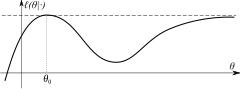
The identification condition is absolutely necessary for the ML estimator to be consistent. When this condition holds, the limiting likelihood function ℓ(θ|·) has unique global maximum at θ0.
Compactness: the parameter space Θ of the model is compact.
The identification condition establishes that the log-likelihood has a unique global maximum. Compactness implies that the likelihood cannot approach the maximum value arbitrarily close at some other point (as demonstrated for example in the picture on the right).
Compactness is only a sufficient condition and not a necessary condition. Compactness can be replaced by some other conditions, such as:
both concavity of the log-likelihood function and compactness of some (nonempty) upper level sets of the log-likelihood function, or
existence of a compact neighborhoodN of θ0 such that outside of N the log-likelihood function is less than the maximum by at least some ε > 0.
Continuity: the function ln f(x | θ) is continuous in θ for almost all values of x:
The continuity here can be replaced with a slightly weaker condition of upper semi-continuity.
Dominance: there exists D(x) integrable with respect to the distribution f(x | θ0) such that
By the uniform law of large numbers, the dominance condition together with continuity establish the uniform convergence in probability of the log-likelihood:
The dominance condition can be employed in the case of i.i.d. observations. In the non-i.i.d. case, the uniform convergence in probability can be checked by showing that the sequence is stochastically equicontinuous. If one wants to demonstrate that the ML estimator converges to θ0 almost surely, then a stronger condition of uniform convergence almost surely has to be imposed:
Additionally, if (as assumed above) the data were generated by , then under certain conditions, it can also be shown that the maximum likelihood estimator converges in distribution to a normal distribution. Specifically,
where I is the Fisher information matrix.
Functional invariance
The maximum likelihood estimator selects the parameter value which gives the observed data the largest possible probability (or probability density, in the continuous case). If the parameter consists of a number of components, then we define their separate maximum likelihood estimators, as the corresponding component of the MLE of the complete parameter. Consistent with this, if is the MLE for , and if is any transformation of , then the MLE for is by definition
It maximizes the so-called profile likelihood:
The MLE is also equivariant with respect to certain transformations of the data. If where is one to one and does not depend on the parameters to be estimated, then the density functions satisfy
and hence the likelihood functions for and differ only by a factor that does not depend on the model parameters.
For example, the MLE parameters of the log-normal distribution are the same as those of the normal distribution fitted to the logarithm of the data.
Efficiency
As assumed above, if the data were generated by then under certain conditions, it can also be shown that the maximum likelihood estimator converges in distribution to a normal distribution. It is √n-consistent and asymptotically efficient, meaning that it reaches the Cramér–Rao bound. Specifically,
where is the Fisher information matrix:
In particular, it means that the bias of the maximum likelihood estimator is equal to zero up to the order 1/√n.
Second-order efficiency after correction for bias
However, when we consider the higher-order terms in the expansion of the distribution of this estimator, it turns out that θmle has bias of order 1⁄n. This bias is equal to (componentwise)
where (with superscripts) denotes the (j,k)-th component of the inverse Fisher information matrix , and
Using these formulae it is possible to estimate the second-order bias of the maximum likelihood estimator, and correct for that bias by subtracting it:
This estimator is unbiased up to the terms of order 1/n, and is called the bias-corrected maximum likelihood estimator.
This bias-corrected estimator is second-order efficient (at least within the curved exponential family), meaning that it has minimal mean squared error among all second-order bias-corrected estimators, up to the terms of the order 1/n2 . It is possible to continue this process, that is to derive the third-order bias-correction term, and so on. However, the maximum likelihood estimator is not third-order efficient.
Relation to Bayesian inference
A maximum likelihood estimator coincides with the most probable Bayesian estimator given a uniform prior distribution on the parameters. Indeed, the maximum a posteriori estimate is the parameter θ that maximizes the probability of θ given the data, given by Bayes' theorem:
where is the prior distribution for the parameter θ and where is the probability of the data averaged over all parameters. Since the denominator is independent of θ, the Bayesian estimator is obtained by maximizing with respect to θ. If we further assume that the prior is a uniform distribution, the Bayesian estimator is obtained by maximizing the likelihood function . Thus the Bayesian estimator coincides with the maximum likelihood estimator for a uniform prior distribution .
Application of maximum-likelihood estimation in Bayes decision theory
In many practical applications in machine learning, maximum-likelihood estimation is used as the model for parameter estimation.
The Bayesian Decision theory is about designing a classifier that minimizes total expected risk, especially, when the costs (the loss function) associated with different decisions are equal, the classifier is minimizing the error over the whole distribution.
Thus, the Bayes Decision Rule is stated as
"decide if otherwise decide "
where are predictions of different classes. From a perspective of minimizing error, it can also be stated as
where
if we decide and if we decide
By applying Bayes' theorem
,
and if we further assume the zero-or-one loss function, which is a same loss for all errors, the Bayes Decision rule can be reformulated as:
where is the prediction and is the prior probability.
Relation to minimizing Kullback–Leibler divergence and cross entropy
Finding that maximizes the likelihood is asymptotically equivalent to finding the that defines a probability distribution () that has a minimal distance, in terms of Kullback–Leibler divergence, to the real probability distribution from which our data were generated (i.e., generated by ). In an ideal world, P and Q are the same (and the only thing unknown is that defines P), but even if they are not and the model we use is misspecified, still the MLE will give us the "closest" distribution (within the restriction of a model Q that depends on ) to the real distribution .
Proof.
For simplicity of notation, let's assume that P=Q. Let there be n i.i.d data samples from some probability , that we try to estimate by finding that will maximize the likelihood using , then:
Where . Using h helps see how we are using the law of large numbers to move from the average of h(x) to the expectancy of it using the law of the unconscious statistician. The first several transitions have to do with laws of logarithm and that finding that maximizes some function will also be the one that maximizes some monotonic transformation of that function (i.e.: adding/multiplying by a constant).
Since cross entropy is just Shannon's entropy plus KL divergence, and since the entropy of is constant, then the MLE is also asymptotically minimizing cross entropy.
Examples
Discrete uniform distribution
Consider a case where n tickets numbered from 1 to n are placed in a box and one is selected at random (see uniform distribution); thus, the sample size is 1. If n is unknown, then the maximum likelihood estimator of n is the number m on the drawn ticket. (The likelihood is 0 for n < m, 1⁄n for n ≥ m, and this is greatest when n = m. Note that the maximum likelihood estimate of n occurs at the lower extreme of possible values {m, m + 1, ...}, rather than somewhere in the "middle" of the range of possible values, which would result in less bias.) The expected value of the number m on the drawn ticket, and therefore the expected value of , is (n + 1)/2. As a result, with a sample size of 1, the maximum likelihood estimator for n will systematically underestimate n by (n − 1)/2.
Discrete distribution, finite parameter space
Suppose one wishes to determine just how biased an unfair coin is. Call the probability of tossing a 'head' p. The goal then becomes to determine p.
Suppose the coin is tossed 80 times: i.e. the sample might be something like x1 = H, x2 = T, ..., x80 = T, and the count of the number of heads "H" is observed.
The probability of tossing tails is 1 − p (so here p is θ above). Suppose the outcome is 49 heads and 31 tails, and suppose the coin was taken from a box containing three coins: one which gives heads with probability p = 1⁄3, one which gives heads with probability p = 1⁄2 and another which gives heads with probability p = 2⁄3. The coins have lost their labels, so which one it was is unknown. Using maximum likelihood estimation, the coin that has the largest likelihood can be found, given the data that were observed. By using the probability mass function of the binomial distribution with sample size equal to 80, number successes equal to 49 but for different values of p (the "probability of success"), the likelihood function (defined below) takes one of three values:
The likelihood is maximized when p = 2⁄3, and so this is the maximum likelihood estimate for p.
Discrete distribution, continuous parameter space
Now suppose that there was only one coin but its p could have been any value 0 ≤ p ≤ 1 . The likelihood function to be maximised is
and the maximisation is over all possible values 0 ≤ p ≤ 1 .
Likelihood function for proportion value of a binomial process (n = 10)
One way to maximize this function is by differentiating with respect to p and setting to zero:
This is a product of three terms. The first term is 0 when p = 0. The second is 0 when p = 1. The third is zero when p = 49⁄80. The solution that maximizes the likelihood is clearly p = 49⁄80 (since p = 0 and p = 1 result in a likelihood of 0). Thus the maximum likelihood estimator for p is 49⁄80.
This result is easily generalized by substituting a letter such as s in the place of 49 to represent the observed number of 'successes' of our Bernoulli trials, and a letter such as n in the place of 80 to represent the number of Bernoulli trials. Exactly the same calculation yields s⁄n which is the maximum likelihood estimator for any sequence of n Bernoulli trials resulting in s 'successes'.
Continuous distribution, continuous parameter space
For the normal distribution which has probability density function
the corresponding probability density function for a sample of n independent identically distributed normal random variables (the likelihood) is
This family of distributions has two parameters: θ = (μ, σ); so we maximize the likelihood, , over both parameters simultaneously, or if possible, individually.
Since the logarithm function itself is a continuous strictly increasing function over the range of the likelihood, the values which maximize the likelihood will also maximize its logarithm (the log-likelihood itself is not necessarily strictly increasing). The log-likelihood can be written as follows:
(Note: the log-likelihood is closely related to information entropy and Fisher information.)
We now compute the derivatives of this log-likelihood as follows.
where is the sample mean. This is solved by
This is indeed the maximum of the function, since it is the only turning point in μ and the second derivative is strictly less than zero. Its expected value is equal to the parameter μ of the given distribution,
which means that the maximum likelihood estimator is unbiased.
Similarly we differentiate the log-likelihood with respect to σ and equate to zero:
which is solved by
Inserting the estimate we obtain
To calculate its expected value, it is convenient to rewrite the expression in terms of zero-mean random variables (statistical error) . Expressing the estimate in these variables yields
Simplifying the expression above, utilizing the facts that and , allows us to obtain
This means that the estimator is biased for . It can also be shown that is biased for , but that both and are consistent.
Formally we say that the maximum likelihood estimator for is
In this case the MLEs could be obtained individually. In general this may not be the case, and the MLEs would have to be obtained simultaneously.
The normal log-likelihood at its maximum takes a particularly simple form:
This maximum log-likelihood can be shown to be the same for more general least squares, even for non-linear least squares. This is often used in determining likelihood-based approximate confidence intervals and confidence regions, which are generally more accurate than those using the asymptotic normality discussed above.
Non-independent variables
It may be the case that variables are correlated, that is, not independent. Two random variables and are independent only if their joint probability density function is the product of the individual probability density functions, i.e.
Suppose one constructs an order-n Gaussian vector out of random variables , where each variable has means given by . Furthermore, let the covariance matrix be denoted by . The joint probability density function of these n random variables then follows a multivariate normal distribution given by:
In the bivariate case, the joint probability density function is given by:
In this and other cases where a joint density function exists, the likelihood function is defined as above, in the section "principles," using this density.
Example
are counts in cells / boxes 1 up to m; each box has a different probability (think of the boxes being bigger or smaller) and we fix the number of balls that fall to be :. The probability of each box is , with a constraint: . This is a case in which the s are not independent, the joint probability of a vector is called the multinomial and has the form:
Each box taken separately against all the other boxes is a binomial and this is an extension thereof.
The log-likelihood of this is:
The constraint has to be taken into account and use the Lagrange multipliers:
By posing all the derivatives to be 0, the most natural estimate is derived
Maximizing log likelihood, with and without constraints, can be an unsolvable problem in closed form, then we have to use iterative procedures.
Iterative procedures
Except for special cases, the likelihood equations
cannot be solved explicitly for an estimator . Instead, they need to be solved iteratively: starting from an initial guess of (say ), one seeks to obtain a convergent sequence . Many methods for this kind of optimization problem are available, but the most commonly used ones are algorithms based on an updating formula of the form
where the vector indicates the descent direction of the rth "step," and the scalar captures the "step length," also known as the learning rate.
(Note: here it is a maximization problem, so the sign before gradient is flipped)
that is small enough for convergence and
Gradient descent method requires to calculate the gradient at the rth iteration, but no need to calculate the inverse of second-order derivative, i.e., the Hessian matrix. Therefore, it is computationally faster than Newton-Raphson method.
where is the score and is the inverse of the Hessian matrix of the log-likelihood function, both evaluated the rth iteration. But because the calculation of the Hessian matrix is computationally costly, numerous alternatives have been proposed. The popular Berndt–Hall–Hall–Hausman algorithm approximates the Hessian with the outer product of the expected gradient, such that
BFGS also gives a solution that is symmetric and positive-definite:
where
BFGS method is not guaranteed to converge unless the function has a quadratic Taylor expansion near an optimum. However, BFGS can have acceptable performance even for non-smooth optimization instances
Another popular method is to replace the Hessian with the Fisher information matrix, , giving us the Fisher scoring algorithm. This procedure is standard in the estimation of many methods, such as generalized linear models.
Although popular, quasi-Newton methods may converge to a stationary point that is not necessarily a local or global maximum, but rather a local minimum or a saddle point. Therefore, it is important to assess the validity of the obtained solution to the likelihood equations, by verifying that the Hessian, evaluated at the solution, is both negative definite and well-conditioned.
Early users of maximum likelihood were Carl Friedrich Gauss, Pierre-Simon Laplace, Thorvald N. Thiele, and Francis Ysidro Edgeworth. However, its widespread use rose between 1912 and 1922 when Ronald Fisher recommended, widely popularized, and carefully analyzed maximum-likelihood estimation (with fruitless attempts at proofs).
Maximum-likelihood estimation finally transcended heuristic justification in a proof published by Samuel S. Wilks in 1938, now called Wilks' theorem. The theorem shows that the error in the logarithm of likelihood values for estimates from multiple independent observations is asymptotically χ 2-distributed, which enables convenient determination of a confidence region around any estimate of the parameters. The only difficult part of Wilks' proof depends on the expected value of the Fisher information matrix, which is provided by a theorem proven by Fisher. Wilks continued to improve on the generality of the theorem throughout his life, with his most general proof published in 1962.
Reviews of the development of maximum likelihood estimation have been provided by a number of authors.
Extremum estimator: a more general class of estimators to which MLE belongs
Fisher information: information matrix, its relationship to covariance matrix of ML estimates
Mean squared error: a measure of how 'good' an estimator of a distributional parameter is (be it the maximum likelihood estimator or some other estimator)
RANSAC: a method to estimate parameters of a mathematical model given data that contains outliers
Rao–Blackwell theorem: yields a process for finding the best possible unbiased estimator (in the sense of having minimal mean squared error); the MLE is often a good starting place for the process
Wilks' theorem: provides a means of estimating the size and shape of the region of roughly equally-probable estimates for the population's parameter values, using the information from a single sample, using a chi-squared distribution
Magnus, Jan R. (2017). "Maximum Likelihood". Introduction to the Theory of Econometrics. Amsterdam, NL: VU University Press. pp. 53–68. ISBN978-90-8659-766-6.
Millar, Russell B. (2011). Maximum Likelihood Estimation and Inference. Hoboken, NJ: Wiley. ISBN978-0-470-09482-2.
Severini, Thomas A. (2000). Likelihood Methods in Statistics. New York, NY: Oxford University Press. ISBN0-19-850650-3.
Ward, Michael D.; Ahlquist, John S. (2018). Maximum Likelihood for Social Science: Strategies for Analysis. Cambridge University Press. ISBN978-1-316-63682-4.
Lesser, Lawrence M. (2007). "'MLE' song lyrics". Mathematical Sciences / College of Science. University of Texas. El Paso, TX. Retrieved 2021-03-06.
This article uses material from the Wikipedia English article Maximum likelihood estimation, which is released under the Creative Commons Attribution-ShareAlike 3.0 license ("CC BY-SA 3.0"); additional terms may apply (view authors). Content is available under CC BY-SA 4.0 unless otherwise noted. Images, videos and audio are available under their respective licenses. ®Wikipedia is a registered trademark of the Wiki Foundation, Inc. Wiki English (DUHOCTRUNGQUOC.VN) is an independent company and has no affiliation with Wiki Foundation.


and


is the maximum likelihood estimator for
is any transformation of
is
. This property is less commonly known as functional equivariance. The invariance property holds for arbitrary transformation
, although the proof simplifies if


if
otherwise decide
"


,


that is small enough for convergence and

and


