Logistic Function
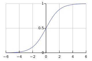
A logistic function or logistic curve is a common S-shaped curve (sigmoid curve) with the equation
where

For values of in the domain of real numbers from to , the S-curve shown on the right is obtained, with the graph of approaching as approaches and approaching zero as approaches .
The logistic function finds applications in a range of fields, including biology (especially ecology), biomathematics, chemistry, demography, economics, geoscience, mathematical psychology, probability, sociology, political science, linguistics, statistics, and artificial neural networks. A generalization of the logistic function is the hyperbolastic function of type I.
The standard logistic function, where , is sometimes simply called the sigmoid. It is also sometimes called the expit, being the inverse of the logit.
History

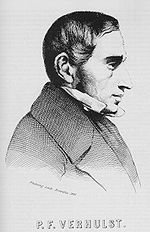
The logistic function was introduced in a series of three papers by Pierre François Verhulst between 1838 and 1847, who devised it as a model of population growth by adjusting the exponential growth model, under the guidance of Adolphe Quetelet. Verhulst first devised the function in the mid 1830s, publishing a brief note in 1838, then presented an expanded analysis and named the function in 1844 (published 1845); the third paper adjusted the correction term in his model of Belgian population growth.
The initial stage of growth is approximately exponential (geometric); then, as saturation begins, the growth slows to linear (arithmetic), and at maturity, growth stops.
Verhulst did not explain the choice of the term "logistic" (French: logistique), but it is presumably in contrast to the logarithmic curve, and by analogy with arithmetic and geometric. His growth model is preceded by a discussion of arithmetic growth and geometric growth (whose curve he calls a logarithmic curve, instead of the modern term exponential curve), and thus "logistic growth" is presumably named by analogy, logistic being from Ancient Greek: λογῐστῐκός, romanized: logistikós, a traditional division of Greek mathematics.
The term is unrelated to the military and management term logistics, which is instead from French: logis "lodgings", though some believe the Greek term also influenced logistics; see Logistics § Origin for details. [citation needed]
Mathematical properties
The standard logistic function is the logistic function with parameters 


In practice, due to the nature of the exponential function 

The logistic function has the symmetry property that

Thus, 
The logistic function is an offset and scaled hyperbolic tangent function:


This follows from

Derivative

The standard logistic function has an easily calculated derivative. The derivative is known as the density of the logistic distribution:


Integral
Conversely, its antiderivative can be computed by the substitution 


In artificial neural networks, this is known as the softplus function and (with scaling) is a smooth approximation of the ramp function, just as the logistic function (with scaling) is a smooth approximation of the Heaviside step function.
Logistic differential equation
The unique standard logistic function is the solution of the simple first-order non-linear ordinary differential equation

with boundary condition 
The qualitative behavior is easily understood in terms of the phase line: the derivative is 0 when the function is 1; and the derivative is positive for 

The logistic equation is a special case of the Bernoulli differential equation and has the following solution:

Choosing the constant of integration 

More quantitatively, as can be seen from the analytical solution, the logistic curve shows early exponential growth for negative argument, which reaches to linear growth of slope 1/4 for an argument near 0, then approaches 1 with an exponentially decaying gap.
The logistic function is the inverse of the natural logit function
and so converts the logarithm of odds into a probability. The conversion from the log-likelihood ratio of two alternatives also takes the form of a logistic curve.
The differential equation derived above is a special case of a general differential equation that only models the sigmoid function for 

 .
. The hyperbolic-tangent relationship leads to another form for the logistic function's derivative:

which ties the logistic function into the logistic distribution.
Rotational symmetry about (0, 1/2)
The sum of the logistic function and its reflection about the vertical axis, 

The logistic function is thus rotationally symmetrical about the point (0, 1/2).
Applications
Link created an extension of Wald's theory of sequential analysis to a distribution-free accumulation of random variables until either a positive or negative bound is first equaled or exceeded. Link derives the probability of first equaling or exceeding the positive boundary as 
In ecology: modeling population growth

A typical application of the logistic equation is a common model of population growth (see also population dynamics), originally due to Pierre-François Verhulst in 1838, where the rate of reproduction is proportional to both the existing population and the amount of available resources, all else being equal. The Verhulst equation was published after Verhulst had read Thomas Malthus' An Essay on the Principle of Population, which describes the Malthusian growth model of simple (unconstrained) exponential growth. Verhulst derived his logistic equation to describe the self-limiting growth of a biological population. The equation was rediscovered in 1911 by A. G. McKendrick for the growth of bacteria in broth and experimentally tested using a technique for nonlinear parameter estimation. The equation is also sometimes called the Verhulst-Pearl equation following its rediscovery in 1920 by Raymond Pearl (1879–1940) and Lowell Reed (1888–1966) of the Johns Hopkins University. Another scientist, Alfred J. Lotka derived the equation again in 1925, calling it the law of population growth.
Letting 


where the constant 

In the equation, the early, unimpeded growth rate is modeled by the first term 


where

where 


In ecology, species are sometimes referred to as 


Integral
The antiderivative of the ecological form of the logistic function can be computed by the substitution 


Time-varying carrying capacity
Since the environmental conditions influence the carrying capacity, as a consequence it can be time-varying, with 

A particularly important case is that of carrying capacity that varies periodically with period 

It can be shown that in such a case, independently from the initial value 


A typical value of 

Another interesting generalization is to consider that the carrying capacity 
In statistics and machine learning
Logistic functions are used in several roles in statistics. For example, they are the cumulative distribution function of the logistic family of distributions, and they are, a bit simplified, used to model the chance a chess player has to beat their opponent in the Elo rating system. More specific examples now follow.
Logistic regression
Logistic functions are used in logistic regression to model how the probability 

where 


Logistic regression and other log-linear models are also commonly used in machine learning. A generalisation of the logistic function to multiple inputs is the softmax activation function, used in multinomial logistic regression.
Another application of the logistic function is in the Rasch model, used in item response theory. In particular, the Rasch model forms a basis for maximum likelihood estimation of the locations of objects or persons on a continuum, based on collections of categorical data, for example the abilities of persons on a continuum based on responses that have been categorized as correct and incorrect.
Neural networks
Logistic functions are often used in artificial neural networks to introduce nonlinearity in the model or to clamp signals to within a specified interval. A popular neural net element computes a linear combination of its input signals, and applies a bounded logistic function as the activation function to the result; this model can be seen as a "smoothed" variant of the classical threshold neuron.
A common choice for the activation or "squashing" functions, used to clip large magnitudes to keep the response of the neural network bounded, is

which is a logistic function.
These relationships result in simplified implementations of artificial neural networks with artificial neurons. Practitioners caution that sigmoidal functions which are antisymmetric about the origin (e.g. the hyperbolic tangent) lead to faster convergence when training networks with backpropagation.
The logistic function is itself the derivative of another proposed activation function, the softplus.
In medicine: modeling of growth of tumors
Another application of logistic curve is in medicine, where the logistic differential equation is used to model the growth of tumors. This application can be considered an extension of the above-mentioned use in the framework of ecology (see also the Generalized logistic curve, allowing for more parameters). Denoting with 


which is of the type

where 
If a chemotherapy is started with a log-kill effect, the equation may be revised to be

where 


i.e. if the average therapy-induced death rate is greater than the baseline proliferation rate, then there is the eradication of the disease. Of course, this is an oversimplified model of both the growth and the therapy (e.g. it does not take into account the phenomenon of clonal resistance).
In medicine: modeling of a pandemic
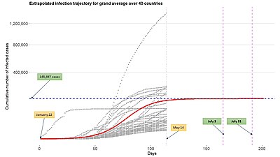
A novel infectious pathogen to which a population has no immunity will generally spread exponentially in the early stages, while the supply of susceptible individuals is plentiful. The SARS-CoV-2 virus that causes COVID-19 exhibited exponential growth early in the course of infection in several countries in early 2020. Factors including a lack of susceptible hosts (through the continued spread of infection until it passes the threshold for herd immunity) or reduction in the accessibility of potential hosts through physical distancing measures, may result in exponential-looking epidemic curves first linearizing (replicating the "logarithmic" to "logistic" transition first noted by Pierre-François Verhulst, as noted above) and then reaching a maximal limit.
A logistic function, or related functions (e.g. the Gompertz function) are usually used in a descriptive or phenomenological manner because they fit well not only to the early exponential rise, but to the eventual levelling off of the pandemic as the population develops a herd immunity. This is in contrast to actual models of pandemics which attempt to formulate a description based on the dynamics of the pandemic (e.g. contact rates, incubation times, social distancing, etc.). Some simple models have been developed, however, which yield a logistic solution.
Modeling early COVID-19 cases

A generalized logistic function, also called the Richards growth curve, has been applied to model the early phase of the COVID-19 outbreak. The authors fit the generalized logistic function to the cumulative number of infected cases, here referred to as infection trajectory. There are different parameterizations of the generalized logistic function in the literature. One frequently used forms is

where 


One of the benefits of using a growth function such as the generalized logistic function in epidemiological modeling is its relatively easy application to the multilevel model framework, where information from different geographic regions can be pooled together.
In chemistry: reaction models
The concentration of reactants and products in autocatalytic reactions follow the logistic function. The degradation of Platinum group metal-free (PGM-free) oxygen reduction reaction (ORR) catalyst in fuel cell cathodes follows the logistic decay function, suggesting an autocatalytic degradation mechanism.
In physics: Fermi–Dirac distribution
The logistic function determines the statistical distribution of fermions over the energy states of a system in thermal equilibrium. In particular, it is the distribution of the probabilities that each possible energy level is occupied by a fermion, according to Fermi–Dirac statistics.
In optics: mirage
The logistic function also finds applications in optics, particularly in modelling phenomena such as mirages. Under certain conditions, such as the presence of a temperature or concentration gradient due to diffusion and balancing with gravity, logistic curve behaviours can emerge.
A mirage, resulting from a temperature gradient that modifies the refractive index related to the density/concentration of the material over distance, can be modelled using a fluid with a refractive index gradient due to the concentration gradient. This mechanism can be equated to a limiting population growth model, where the concentrated region attempts to diffuse into the lower concentration region, while seeking equilibrium with gravity, thus yielding a logistic function curve.
In material science: Phase diagrams
See Diffusion bonding.
In linguistics: language change
In linguistics, the logistic function can be used to model language change: an innovation that is at first marginal begins to spread more quickly with time, and then more slowly as it becomes more universally adopted.
In agriculture: modeling crop response
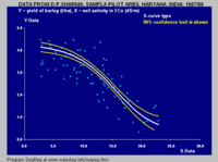
The logistic S-curve can be used for modeling the crop response to changes in growth factors. There are two types of response functions: positive and negative growth curves. For example, the crop yield may increase with increasing value of the growth factor up to a certain level (positive function), or it may decrease with increasing growth factor values (negative function owing to a negative growth factor), which situation requires an inverted S-curve.
In economics and sociology: diffusion of innovations
The logistic function can be used to illustrate the progress of the diffusion of an innovation through its life cycle.
In The Laws of Imitation (1890), Gabriel Tarde describes the rise and spread of new ideas through imitative chains. In particular, Tarde identifies three main stages through which innovations spread: the first one corresponds to the difficult beginnings, during which the idea has to struggle within a hostile environment full of opposing habits and beliefs; the second one corresponds to the properly exponential take-off of the idea, with 

In a sovereign state, the subnational units (constituent states or cities) may use loans to finance their projects. However, this funding source is usually subject to strict legal rules as well as to economy scarcity constraints, especially the resources the banks can lend (due to their equity or Basel limits). These restrictions, which represent a saturation level, along with an exponential rush in an economic competition for money, create a public finance diffusion of credit pleas and the aggregate national response is a sigmoid curve.
Historically, when new products are introduced there is an intense amount of research and development which leads to dramatic improvements in quality and reductions in cost. This leads to a period of rapid industry growth. Some of the more famous examples are: railroads, incandescent light bulbs, electrification, cars and air travel. Eventually, dramatic improvement and cost reduction opportunities are exhausted, the product or process are in widespread use with few remaining potential new customers, and markets become saturated.
Logistic analysis was used in papers by several researchers at the International Institute of Applied Systems Analysis (IIASA). These papers deal with the diffusion of various innovations, infrastructures and energy source substitutions and the role of work in the economy as well as with the long economic cycle. Long economic cycles were investigated by Robert Ayres (1989). Cesare Marchetti published on long economic cycles and on diffusion of innovations. Arnulf Grübler's book (1990) gives a detailed account of the diffusion of infrastructures including canals, railroads, highways and airlines, showing that their diffusion followed logistic shaped curves.
Carlota Perez used a logistic curve to illustrate the long (Kondratiev) business cycle with the following labels: beginning of a technological era as irruption, the ascent as frenzy, the rapid build out as synergy and the completion as maturity.
See also
Notes
References
External links

- L.J. Linacre, Why logistic ogive and not autocatalytic curve?, accessed 2009-09-12.
- https://web.archive.org/web/20060914155939/http://luna.cas.usf.edu/~mbrannic/files/regression/Logistic.html
- Weisstein, Eric W. "Sigmoid Function". MathWorld.
- Online experiments with JSXGraph
- Esses are everywhere.
- Seeing the s-curve is everything.
- Restricted Logarithmic Growth with Injection
This article uses material from the Wikipedia English article Logistic function, which is released under the Creative Commons Attribution-ShareAlike 3.0 license ("CC BY-SA 3.0"); additional terms may apply (view authors). Content is available under CC BY-SA 4.0 unless otherwise noted. Images, videos and audio are available under their respective licenses.
®Wikipedia is a registered trademark of the Wiki Foundation, Inc. Wiki English (DUHOCTRUNGQUOC.VN) is an independent company and has no affiliation with Wiki Foundation.


